
| Version 3 (modified by , 11 years ago) (diff) |
|---|
F. Analyze

In Section F we went through the exercise of retrieving data from iRODS to a local computer. In this Section, we will introduce two different methods that can be used to analyze the measurement data. Analysis of measurement data obtained with OMF/OML is not limited to these two methods, we simply use them for demonstration purposes.
G.1 R Scripts
One potential way to visualize the data is making use of R, which provides a visualization language. For this tutorial, we have create a set of R scripts, which we briefly discuss in the following.
The first R script creates a plot of the RTTs for each ping that's carried out in the experiment in the initial experiment we ran in the tutorial.
library(RSQLite)
con <- dbConnect(dbDriver("SQLite"), dbname = "gimi20-2012-10-18t14.03.42-04.00.sq3")
dbListTables(con)
dbReadTable(con,"pingmonitor_myping")

mydata1 <- dbGetQuery(con, "select dest_addr, rtt from pingmonitor_myping where dest_addr='192.168.4.10'")
rtt1 <- abs(mydata1$rtt)

mydata2 <- dbGetQuery(con, "select dest_addr, rtt from pingmonitor_myping where dest_addr='192.168.5.12'")
rtt2 <- abs(mydata2$rtt)

mydata3 <- dbGetQuery(con, "select dest_addr, rtt from pingmonitor_myping where dest_addr='192.168.4.11'")
rtt3 <- abs(mydata3$rtt)

mydata4 <- dbGetQuery(con, "select dest_addr, rtt from pingmonitor_myping where dest_addr='192.168.2.12'")
rtt4 <- abs(mydata4$rtt)

mydata5 <- dbGetQuery(con, "select dest_addr, rtt from pingmonitor_myping where dest_addr='192.168.1.13'")
rtt5 <- abs(mydata5$rtt)

mydata6 <- dbGetQuery(con, "select dest_addr, rtt from pingmonitor_myping where dest_addr='192.168.5.11'")
rtt6 <- abs(mydata6$rtt)

mydata7 <- dbGetQuery(con, "select dest_addr, rtt from pingmonitor_myping where dest_addr='192.168.2.10'")
rtt7 <- abs(mydata7$rtt)

mydata8 <- dbGetQuery(con, "select dest_addr, rtt from pingmonitor_myping where dest_addr='192.168.3.13'")
rtt8 <- abs(mydata8$rtt)

mydata9 <- dbGetQuery(con, "select dest_addr, rtt from pingmonitor_myping where dest_addr='192.168.6.14'")
rtt9 <- abs(mydata9$rtt)

mydata10 <- dbGetQuery(con, "select dest_addr, rtt from pingmonitor_myping where dest_addr='192.168.1.10'")
rtt10 <- abs(mydata10$rtt)

mydata11 <- dbGetQuery(con, "select dest_addr, rtt from pingmonitor_myping where dest_addr='192.168.3.12'")
rtt11 <- abs(mydata11$rtt)

mydata12 <- dbGetQuery(con, "select dest_addr, rtt from pingmonitor_myping where dest_addr='192.168.6.12'")
rtt12 <- abs(mydata12$rtt)

png(filename="gimi20-nmetrics-eth", height=650, width=900,
 bg="white")
g_range <- range(0,rtt1,rtt2,rtt3,rtt4,rtt5,rtt6,rtt7,rtt8,rtt9,rtt10,rtt11,rtt12)

plot(rtt1,type="o",col="red",ylim= g_range, lty=2, xlab="Experiment Interval",ylab="RTT")
lines(rtt2,type="o",col="blue",xlab="Experiment Interval",ylab="Received Data")
lines(rtt3,type="o",col="green",xlab="Experiment Interval",ylab="Received Data")
lines(rtt4,type="o",col="purple",xlab="Experiment Interval",ylab="Received Data")
lines(rtt5,type="o",col="violetred",xlab="Experiment Interval",ylab="Received Data")
lines(rtt6,type="o",col="springgreen",xlab="Experiment Interval",ylab="Received Data")
lines(rtt7,type="o",col="skyblue",xlab="Experiment Interval",ylab="Received Data")
lines(rtt8,type="o",col="sienna",xlab="Experiment Interval",ylab="Received Data")
lines(rtt9,type="o",col="pink",xlab="Experiment Interval",ylab="Received Data")
lines(rtt10,type="o",col="yellow",xlab="Experiment Interval",ylab="Received Data")
lines(rtt11,type="o",col="thistle",xlab="Experiment Interval",ylab="Received Data")
lines(rtt12,type="o",col="orange",xlab="Experiment Interval",ylab="Received Data")

title(main="nmetrics experiment on ExoGENI (Received Data)", col.main="red", font.main=4)
legend("topright", g_range[4], legend=c("192.168.4.10","192.168.5.12","192.168.4.11","192.168.2.12","192.168.5.11","192.168.2.10","192.168.3.13","192.168.6.14","192.168.1.10","192.168.3.12","192.168.6.12"), cex=0.8,
   col=c("blue","red","green","purple","violetred","springgreen","skyblue","sienna","pink","yellow","thistle","orange"), pch=15:16:17:18:19:20:21:22:23:24:25:26, lty=1:2:3:4:5:6:7:8:9:10:11:12);

dev.off()
The resulting plot is shown below.

The following R script plots otr results from the 4th experiment we executed in Section C.
library(RSQLite)
con <- dbConnect(dbDriver("SQLite"), dbname = "gimi20-otg-nmetrics.sq3")
dbListTables(con)
dbReadTable(con,"otr2_udp_in")

mydata1 <- dbGetQuery(con, "select oml_sender_id, pkt_length from otr2_udp_in where src_host='192.168.4.10'")
pkt_length <- mydata1$pkt_length
#plot(rx_bytes1, type="o", color="red", xlab="Experiment Interval", ylab="Received data")


png(filename="gimi20_otg1.png", height=650, width=900,
 bg="white")
g_range <- range(0,pkt_length)

plot(pkt_length,type="o",col="red",ylim= g_range, lty=2, xlab="Experiment Interval",ylab="Packet Size")

title(main="Received packet size with sender address 192.168.4.10", col.main="red", font.main=4)
legend("bottomright", g_range[1], legend=c("interface1"), cex=0.8,
   col=c("blue"), pch=21, lty=1);

dev.off()
The resulting plot is shown below.

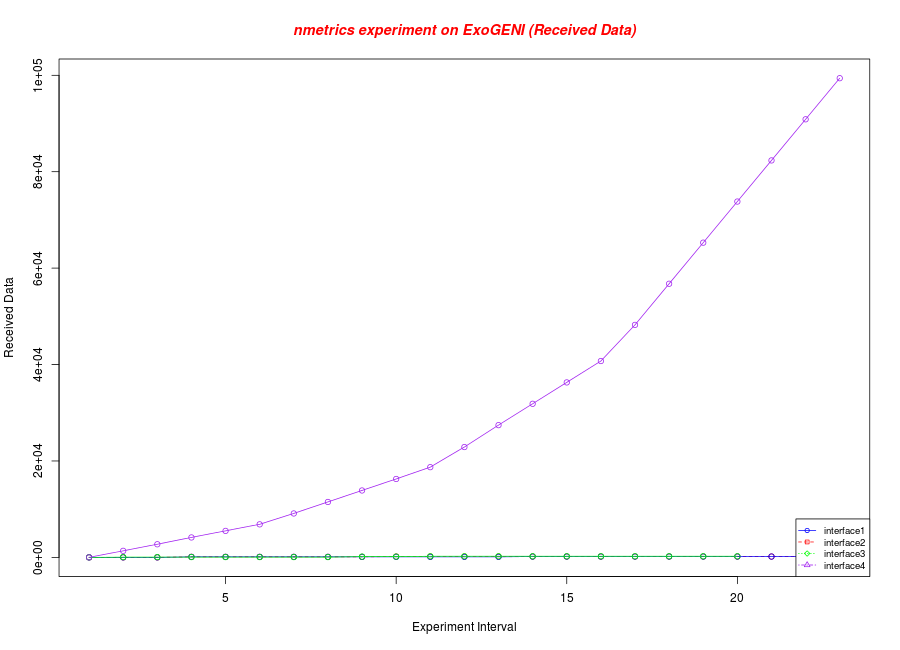
The following script plots part of nmetrics results from the 4th experiment we executed.
library(RSQLite)
con <- dbConnect(dbDriver("SQLite"), dbname = "gimi20-otg-nmetrics.sq3")
dbListTables(con)
dbReadTable(con,"nmetrics_net_if")

mydata1 <- dbGetQuery(con, "select oml_sender_id, rx_bytes from nmetrics_net_if where oml_sender_id=1")
rx_bytes1 <- abs(mydata1$rx_bytes)
#plot(rx_bytes1, type="o", color="red", xlab="Experiment Interval", ylab="Received data")

mydata2 <- dbGetQuery(con, "select oml_sender_id, rx_bytes from nmetrics_net_if where oml_sender_id=2")
rx_bytes2 <- abs(mydata2$rx_bytes)

mydata3 <- dbGetQuery(con, "select oml_sender_id, rx_bytes from nmetrics_net_if where oml_sender_id=3")
rx_bytes3 <- abs(mydata3$rx_bytes)

mydata4 <- dbGetQuery(con, "select oml_sender_id, rx_bytes from nmetrics_net_if where oml_sender_id=4")
rx_bytes4 <- abs(mydata4$rx_bytes)

png(filename="gimi20-nmetrics-eth", height=650, width=900,
 bg="white")
g_range <- range(0,rx_bytes1,rx_bytes2,rx_bytes3,rx_bytes4)

plot(rx_bytes1,type="o",col="red",ylim= g_range, lty=2, xlab="Experiment Interval",ylab="Received Data")
lines(rx_bytes2,type="o",col="blue",xlab="Experiment Interval",ylab="Received Data")
lines(rx_bytes3,type="o",col="green",xlab="Experiment Interval",ylab="Received Data")
lines(rx_bytes4,type="o",col="purple",xlab="Experiment Interval",ylab="Received Data")
title(main="nmetrics experiment on ExoGENI (Received Data)", col.main="red", font.main=4)
legend("bottomright", g_range[4], legend=c("interface1","interface2","interface3","interface4"), cex=0.8,
   col=c("blue","red","green","purple"), pch=21:22:23:24, lty=1:2:3:4);
The resulting plot is shown below.

All three scripts are simply executed with:
R -f <script_name>
The benefit of using R scripts is that they can produce graphs that can be used in documents!
The results can then be stored into iRODS using the itools presented in Section E.2.
G.2 omf_web
The second alternative we use in the tutorial is omf_web, which already has been presented in Section D.
Attachments (3)
- gimi20-nmetrics-eth.png (31.6 KB) - added by 11 years ago.
- gimi20-ping.png (42.9 KB) - added by 11 years ago.
- gimi20_otg1.png (29.8 KB) - added by 11 years ago.
Download all attachments as: .zip