
| Version 7 (modified by , 11 years ago) (diff) |
|---|
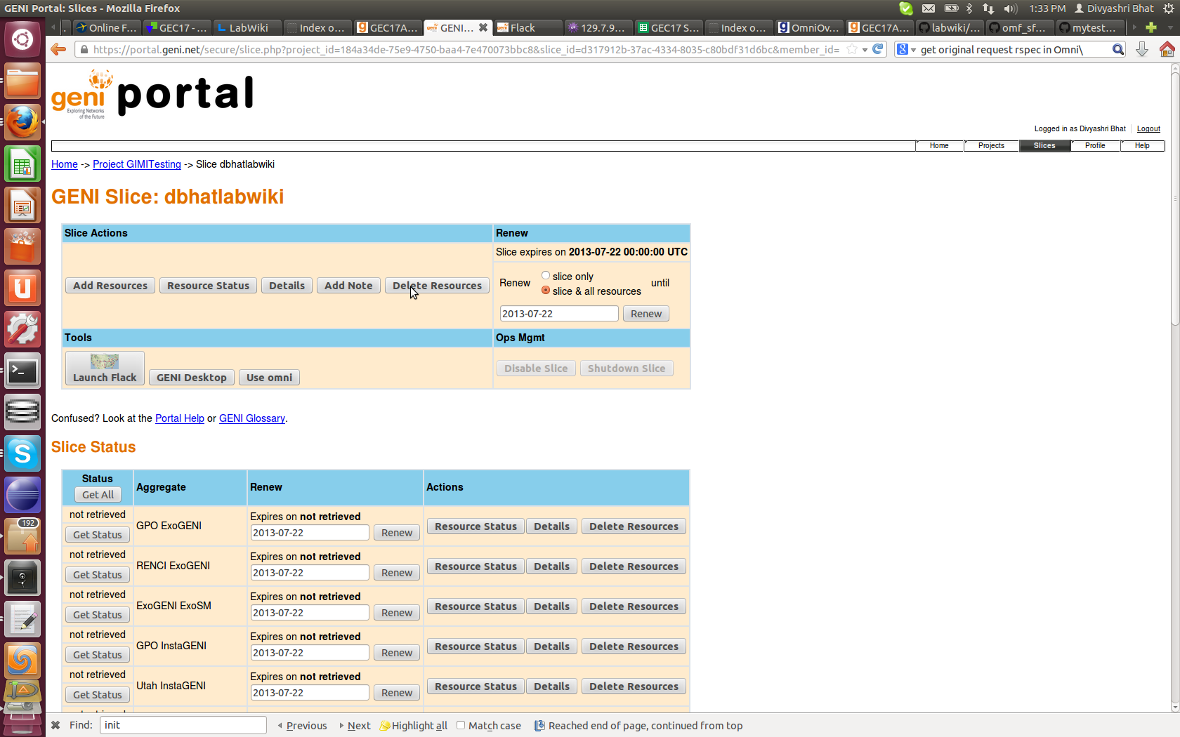
Finish
E. Push to iRODS
E.1 Overview
In GIMI, iRODS is used as the repository for measurement data. At the moment our iRODS data system consist of three servers (RENCI, NICTA, and UMass) and a metadata catalog (located at RENCI).
E.2 Storing data on iRODS
- After successful completion of an experiment the measurement data from the experiment have been stored in iRODS. We will now look into two options on how this data can be handled.
E.2.1 iRODS command line tools in the user work space
- The GENI User Workspace comes already with the iRODS command line tools installed.
- If you have not done so far use iinit to create a file that contains your iRODS password in a scrambled form. This will then be used automatically by the icommands for authentication with the server.
$ iinit
You will be prompted for a password. Please enter the one given on the paper handout.
- The iRODS client uses a configuration file (~/.irods/.irodsEnv) that sets certain parameter for the icommands. Here is and example:
# iRODS personal configuration file.
#
# This file was automatically created during iRODS installation.
#   Created Thu Feb 16 14:06:27 2012
#
# iRODS server host name:
irodsHost 'emmy9.casa.umass.edu'
# iRODS server port number:
irodsPort 1247

# Default storage resource name:
irodsDefResource 'iRODSUmass2'
# Home directory in iRODS:
irodsHome '/geniRenci/home/gimiXX'
# Current directory in iRODS:
irodsCwd '/geniRenci/home/gimiXX'
# Account name:
irodsUserName 'gimiXX'
# Zone:
irodsZone 'geniRenci'
- Retrieve file from your iRODS home directory into user workspace.
$ iget <file_name>
Assuming you wanted to retrieve a file called gimitesting.sq3 the command would look as follows:
$ iget gimitesting.sq3
- Store data from user workspace into your iRODS home directory.
$ iput <file_name>
- Add metadata information to stored file.
$ imeta add -d <file_name> <name> <value> <unit>
For example if you wanted to add the slice name of the experiment as metadata for file gimi01-ping_all.sq3, the command would look as follows:$ imeta add -d gimi01-ping_all.sq3 SliceName gimi01
(<unit> is not required.)
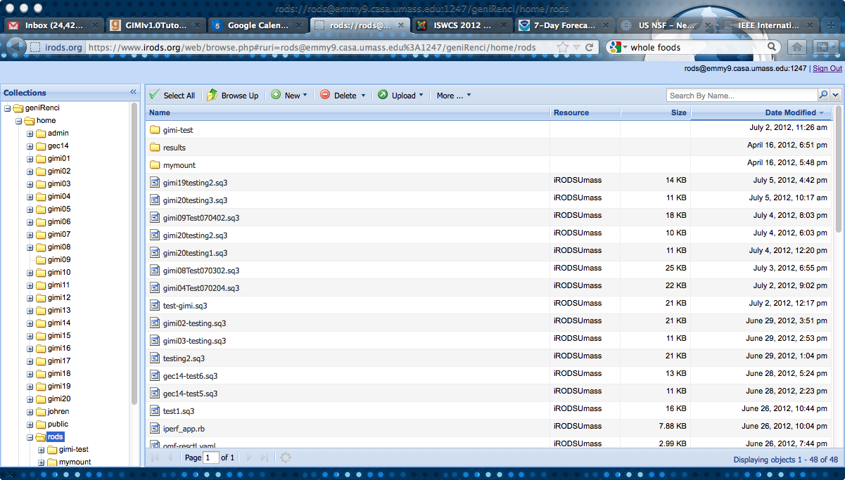
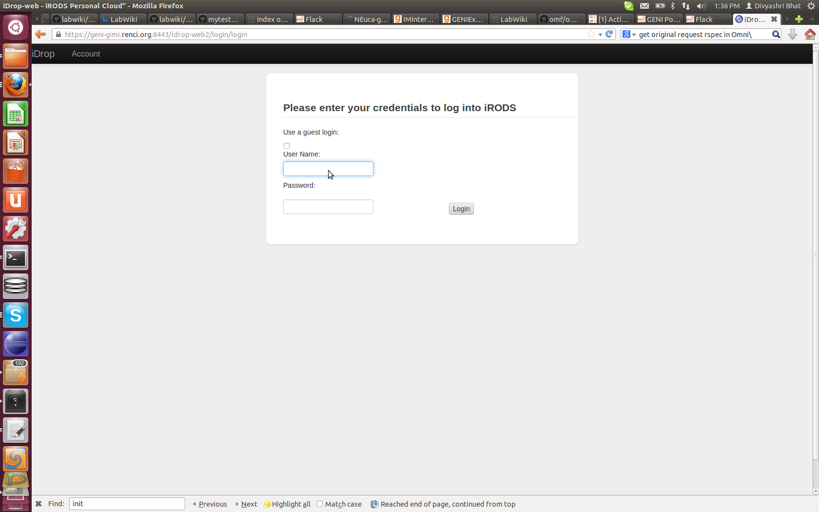
E.2.2 iRODS web interface
iRODS also provides a nice and easy to use web interface, which we will explore in the following.
- Point the browser in your user workspace to the following link: https://www.irods.org/web/index.php
- Input the following information to sign in:
Host/IP: emmy9.casa.umass.edu
Port: 1247
Username: as given on printout
Password: as given on printout
- The following screenshot shows an example for the web interface:

E.3 IRODS and OML
In GIMI we have enabled an option in OML2.8 that allows the execution of script. We use this functionality to automatically save measurement results in IRODS after a measurement has successfully completed.
E.4 DISCLAIMER
The iRODS service we are offering within the scope of GIMI does NOT guarantee 100% reliable data storage (i.e., we do NOT back up the data). If you are performing your own experiments and want to use iRODS you are absolutely welcome but be aware that we do NOT guarantee recovery from data loss.
In Section F we went through the exercise of retrieving data from iRODS to a local computer. In this Section, we will introduce two different methods that can be used to analyze the measurement data. Analysis of measurement data obtained with OMF/OML is not limited to these two methods, we simply use them for demonstration purposes.
G.1 R Scripts
One potential way to visualize the data is making use of R, which provides a visualization language. For this tutorial, we have create a set of R scripts, which we briefly discuss in the following.
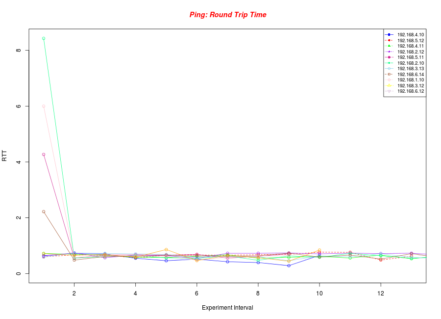
The first R script creates a plot of the RTTs for each ping that's carried out in the experiment in the initial experiment we ran in the tutorial.
library(RSQLite)
con <- dbConnect(dbDriver("SQLite"), dbname = "gimi20-2012-10-18t14.03.42-04.00.sq3")
dbListTables(con)
dbReadTable(con,"pingmonitor_myping")

mydata1 <- dbGetQuery(con, "select dest_addr, rtt from pingmonitor_myping where dest_addr='192.168.4.10'")
rtt1 <- abs(mydata1$rtt)

mydata2 <- dbGetQuery(con, "select dest_addr, rtt from pingmonitor_myping where dest_addr='192.168.5.12'")
rtt2 <- abs(mydata2$rtt)

mydata3 <- dbGetQuery(con, "select dest_addr, rtt from pingmonitor_myping where dest_addr='192.168.4.11'")
rtt3 <- abs(mydata3$rtt)

mydata4 <- dbGetQuery(con, "select dest_addr, rtt from pingmonitor_myping where dest_addr='192.168.2.12'")
rtt4 <- abs(mydata4$rtt)

mydata5 <- dbGetQuery(con, "select dest_addr, rtt from pingmonitor_myping where dest_addr='192.168.1.13'")
rtt5 <- abs(mydata5$rtt)

mydata6 <- dbGetQuery(con, "select dest_addr, rtt from pingmonitor_myping where dest_addr='192.168.5.11'")
rtt6 <- abs(mydata6$rtt)

mydata7 <- dbGetQuery(con, "select dest_addr, rtt from pingmonitor_myping where dest_addr='192.168.2.10'")
rtt7 <- abs(mydata7$rtt)

mydata8 <- dbGetQuery(con, "select dest_addr, rtt from pingmonitor_myping where dest_addr='192.168.3.13'")
rtt8 <- abs(mydata8$rtt)

mydata9 <- dbGetQuery(con, "select dest_addr, rtt from pingmonitor_myping where dest_addr='192.168.6.14'")
rtt9 <- abs(mydata9$rtt)

mydata10 <- dbGetQuery(con, "select dest_addr, rtt from pingmonitor_myping where dest_addr='192.168.1.10'")
rtt10 <- abs(mydata10$rtt)

mydata11 <- dbGetQuery(con, "select dest_addr, rtt from pingmonitor_myping where dest_addr='192.168.3.12'")
rtt11 <- abs(mydata11$rtt)

mydata12 <- dbGetQuery(con, "select dest_addr, rtt from pingmonitor_myping where dest_addr='192.168.6.12'")
rtt12 <- abs(mydata12$rtt)

png(filename="gimi20-nmetrics-eth", height=650, width=900,
 bg="white")
g_range <- range(0,rtt1,rtt2,rtt3,rtt4,rtt5,rtt6,rtt7,rtt8,rtt9,rtt10,rtt11,rtt12)

plot(rtt1,type="o",col="red",ylim= g_range, lty=2, xlab="Experiment Interval",ylab="RTT")
lines(rtt2,type="o",col="blue",xlab="Experiment Interval",ylab="Received Data")
lines(rtt3,type="o",col="green",xlab="Experiment Interval",ylab="Received Data")
lines(rtt4,type="o",col="purple",xlab="Experiment Interval",ylab="Received Data")
lines(rtt5,type="o",col="violetred",xlab="Experiment Interval",ylab="Received Data")
lines(rtt6,type="o",col="springgreen",xlab="Experiment Interval",ylab="Received Data")
lines(rtt7,type="o",col="skyblue",xlab="Experiment Interval",ylab="Received Data")
lines(rtt8,type="o",col="sienna",xlab="Experiment Interval",ylab="Received Data")
lines(rtt9,type="o",col="pink",xlab="Experiment Interval",ylab="Received Data")
lines(rtt10,type="o",col="yellow",xlab="Experiment Interval",ylab="Received Data")
lines(rtt11,type="o",col="thistle",xlab="Experiment Interval",ylab="Received Data")
lines(rtt12,type="o",col="orange",xlab="Experiment Interval",ylab="Received Data")

title(main="nmetrics experiment on ExoGENI (Received Data)", col.main="red", font.main=4)
legend("topright", g_range[4], legend=c("192.168.4.10","192.168.5.12","192.168.4.11","192.168.2.12","192.168.5.11","192.168.2.10","192.168.3.13","192.168.6.14","192.168.1.10","192.168.3.12","192.168.6.12"), cex=0.8,
   col=c("blue","red","green","purple","violetred","springgreen","skyblue","sienna","pink","yellow","thistle","orange"), pch=15:16:17:18:19:20:21:22:23:24:25:26, lty=1:2:3:4:5:6:7:8:9:10:11:12);

dev.off()
The resulting plot is shown below.

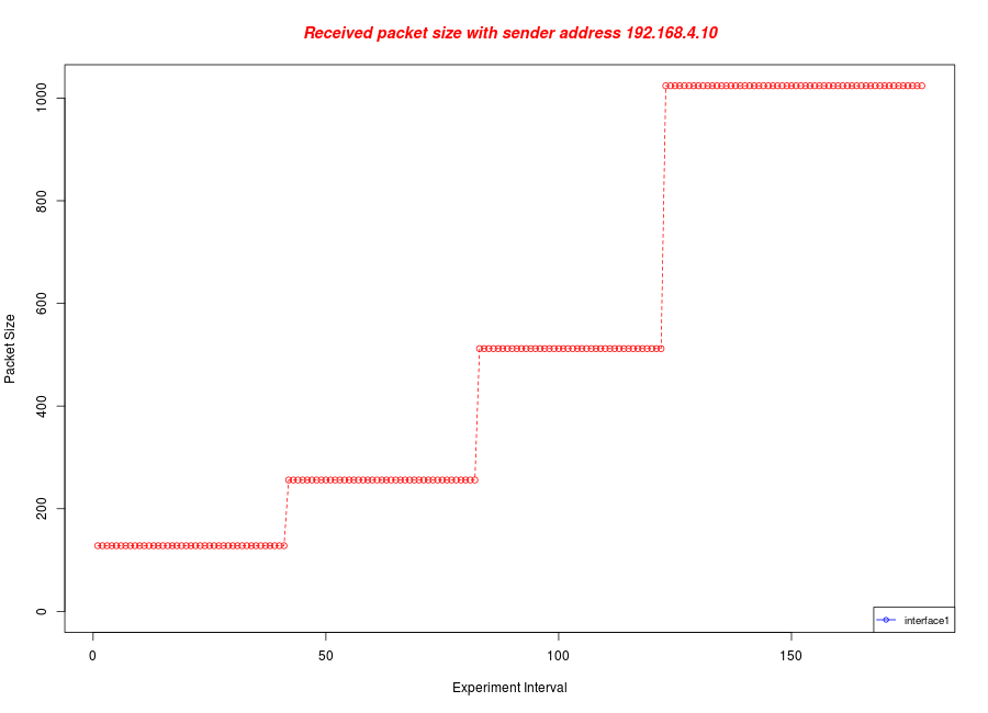
The following R script plots otr results from the 4th experiment we executed in Section C.
library(RSQLite)
con <- dbConnect(dbDriver("SQLite"), dbname = "gimi20-otg-nmetrics.sq3")
dbListTables(con)
dbReadTable(con,"otr2_udp_in")

mydata1 <- dbGetQuery(con, "select oml_sender_id, pkt_length from otr2_udp_in where src_host='192.168.4.10'")
pkt_length <- mydata1$pkt_length
#plot(rx_bytes1, type="o", color="red", xlab="Experiment Interval", ylab="Received data")


png(filename="gimi20_otg1.png", height=650, width=900,
 bg="white")
g_range <- range(0,pkt_length)

plot(pkt_length,type="o",col="red",ylim= g_range, lty=2, xlab="Experiment Interval",ylab="Packet Size")

title(main="Received packet size with sender address 192.168.4.10", col.main="red", font.main=4)
legend("bottomright", g_range[1], legend=c("interface1"), cex=0.8,
   col=c("blue"), pch=21, lty=1);

dev.off()
The resulting plot is shown below.

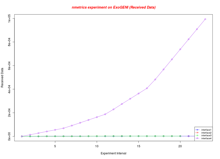
The following script plots part of nmetrics results from the 4th experiment we executed.
library(RSQLite)
con <- dbConnect(dbDriver("SQLite"), dbname = "gimi20-otg-nmetrics.sq3")
dbListTables(con)
dbReadTable(con,"nmetrics_net_if")

mydata1 <- dbGetQuery(con, "select oml_sender_id, rx_bytes from nmetrics_net_if where oml_sender_id=1")
rx_bytes1 <- abs(mydata1$rx_bytes)
#plot(rx_bytes1, type="o", color="red", xlab="Experiment Interval", ylab="Received data")

mydata2 <- dbGetQuery(con, "select oml_sender_id, rx_bytes from nmetrics_net_if where oml_sender_id=2")
rx_bytes2 <- abs(mydata2$rx_bytes)

mydata3 <- dbGetQuery(con, "select oml_sender_id, rx_bytes from nmetrics_net_if where oml_sender_id=3")
rx_bytes3 <- abs(mydata3$rx_bytes)

mydata4 <- dbGetQuery(con, "select oml_sender_id, rx_bytes from nmetrics_net_if where oml_sender_id=4")
rx_bytes4 <- abs(mydata4$rx_bytes)

png(filename="gimi20-nmetrics-eth", height=650, width=900,
 bg="white")
g_range <- range(0,rx_bytes1,rx_bytes2,rx_bytes3,rx_bytes4)

plot(rx_bytes1,type="o",col="red",ylim= g_range, lty=2, xlab="Experiment Interval",ylab="Received Data")
lines(rx_bytes2,type="o",col="blue",xlab="Experiment Interval",ylab="Received Data")
lines(rx_bytes3,type="o",col="green",xlab="Experiment Interval",ylab="Received Data")
lines(rx_bytes4,type="o",col="purple",xlab="Experiment Interval",ylab="Received Data")
title(main="nmetrics experiment on ExoGENI (Received Data)", col.main="red", font.main=4)
legend("bottomright", g_range[4], legend=c("interface1","interface2","interface3","interface4"), cex=0.8,
   col=c("blue","red","green","purple"), pch=21:22:23:24, lty=1:2:3:4);
The resulting plot is shown below.

All three scripts are simply executed with:
R -f <script_name>
The benefit of using R scripts is that they can produce graphs that can be used in documents!
The results can then be stored into iRODS using the itools presented in Section E.2.
G.2 omf_web
The second alternative we use in the tutorial is omf_web, which already has been presented in Section D.
F.1 iRODS Environment Settings
If you haven't already performed this step in A.1, you first have to configure the your local iRODS environment:
- The iRODS client uses a configuration file (~/.irods/.irodsEnv) that sets certain parameter for the icommands. Here is and example:
# iRODS personal configuration file.
#
# This file was automatically created during iRODS installation.
#   Created Thu Feb 16 14:06:27 2012
#
# iRODS server host name:
irodsHost 'emmy9.casa.umass.edu'
# iRODS server port number:
irodsPort 1247

# Default storage resource name:
irodsDefResource 'iRODSUmass2'
# Home directory in iRODS:
irodsHome '/geniRenci/home/gimiXX'
# Current directory in iRODS:
irodsCwd '/geniRenci/home/gimiXX'
# Account name:
irodsUserName 'gimiXX'
# Zone:
irodsZone 'geniRenci'
- First of all copy the iRODS configuration file to .irodsEnv with the following command (replace gimiXX with your username):
$ cp ~/Tutorials/GIMI/gimiXX/gimiXXIrodsEnv ~/.irods/.irodsEnv
- Register with iRODS server by issuing the following command (more details on iRODS will be given shortly):
$ iinit
- You will be prompted for a password. Please type in the password you were provided with on the paper handout!!
F.2 Retrieving Data from iRODS to Local System
In the following we list the steps and commands that will allow you to retrieve data from the iRODS storage to your local storage:
- List content of your home directory
$ ils
- To change to a different directory use
$ icd
- Retrieve file from your iRODS home directory into user workspace.
$ iget <file_name>
Assuming you wanted to retrieve a file called gimitesting.sq3 the command would look as follows:
$ iget gimitesting.sq3
- A complete overview on the iRODS commands can be found here.
F.3 Searching the Catalogue for Data
$ imeta qu -d SliceName like gimi28
Attachments (7)
- irods_screen.png (350.9 KB) - added by 11 years ago.
- gimi20-ping.png (42.9 KB) - added by 11 years ago.
- gimi20-nmetrics-eth.png (31.6 KB) - added by 11 years ago.
- gimi20_otg1.png (29.8 KB) - added by 11 years ago.
- Flack4.png (128.4 KB) - added by 11 years ago.
- deleteresources.png (289.0 KB) - added by 11 years ago.
- iDroplogin.png (158.6 KB) - added by 11 years ago.
Download all attachments as: .zip